Reverse engineering theYouTubeAlgorithm.

For over a decade, the YouTube algorithm has been treated as a black box that creators try to appease and viewers blindly follow. However, in 2016, Google published a paper titled “Deep Neural Networks for YouTube Recommendations” that served as a public technical starting point.

This post attempts to trace the evolutionary path from that 2016 snapshot to the present day. By analyzing the trajectory of AI research - specifically the introduction of Attention mechanisms, Contrastive Learning, Multigate Mixture-of-Experts (MMoE), and finally, Multimodal Large Language Models, we can construct a highly probable blueprint of how the modern recommendation system functions.

Disclaimer: The following is a theoretical framework based on technical clues, published papers, and empirical testing. It is a reverse-engineering hypothesis, not an official documentation.

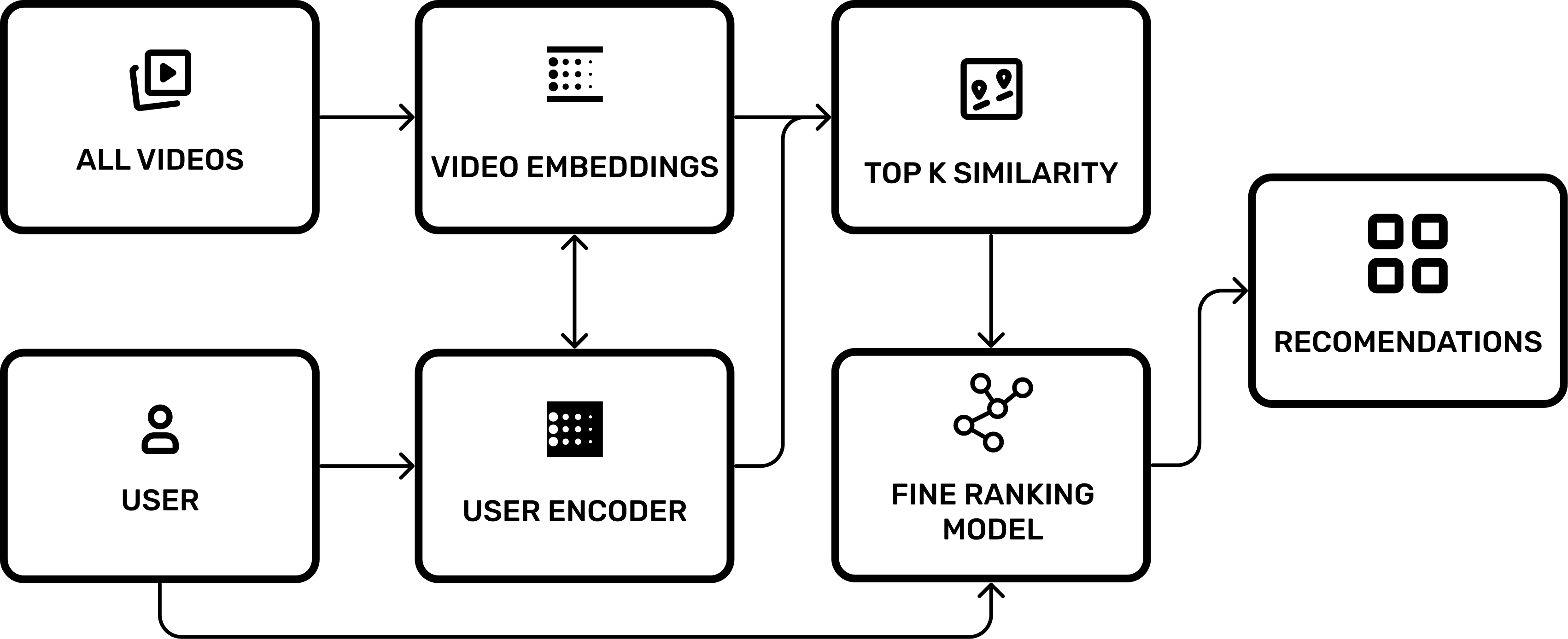
The core problem of recommendation at YouTube’s scale is the “Needle in a Haystack” paradox. You have a user with a specific history, and you have billions of videos. Running a complex predictive model on every single video for every single user visit is computationally impossible.

The 2016 paper revealed that YouTube solves this via a Two-Stage Funnel:

1. Candidate Generation (Recall): Filtering billions of videos down to a few hundred relevant ones.

2. Ranking (Precision): Scoring those few hundred videos with high precision to determine the final order.

Once the system has filtered billions of videos down to a few hundred candidates, it passes them to the Fine Ranking Model. This is where the heavy lifting happens.

In 2016, this was a deep Feed-Forward Network (FFN) designed to predict a single metric: Expected Watch Time.

The Inputs

The model consumes a rich set of features for each candidate video:

• Impression Video ID: The specific video being scored.

• User Language & Video Language: To ensure compatibility.

• Time Since Last Watch: Crucially, this isn’t just the last time you watched this video, but the last time you watched a video semantically similar to it. This allows the model to learn cadence (e.g., learning that you watch “Daily News” every 24 hours, but “Minecraft Let’s Plays” only on weekends).

• Previous Impressions: How many times has the user ignored this video? (A strong negative signal).

• Video and user embeddings

The Objective Function

The model uses Weighted Logistic Regression.
It does not predict “Will the user click?” (CTR). It predicts Expected Watch Time per Impression.

This is why clickbait (high clicks, low duration) eventually gets penalized, while engaging content promotes higher rankings.

Original article figure

In 2017, Google released “Attention Is All You Need,” birthing the Transformer architecture. This likely marked the first massive shift in the algorithm.

Solving the Cold Start with Dual Encoders

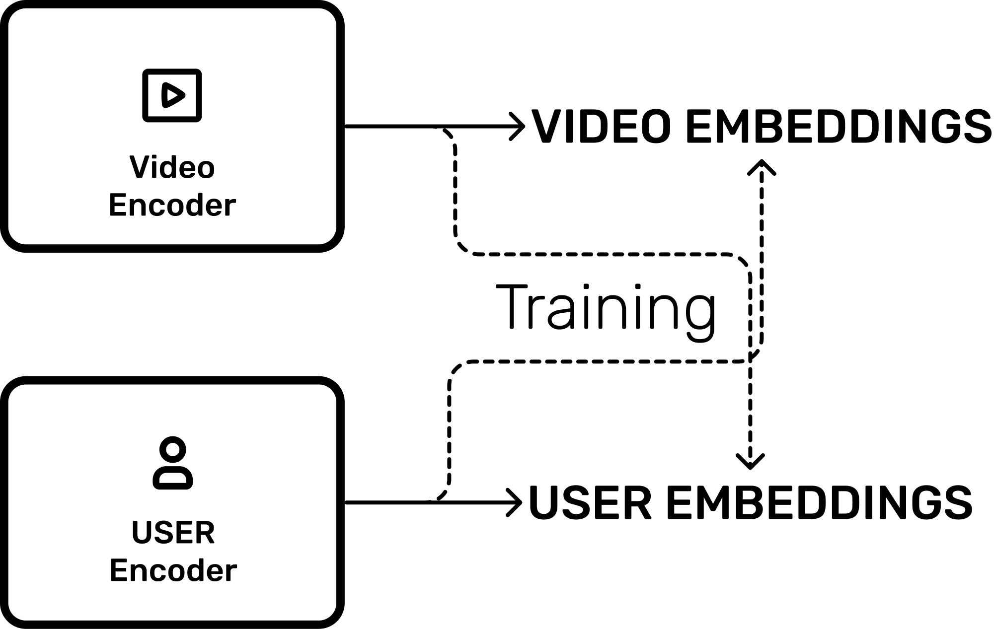
To solve the Cold Start problem, YouTube likely integrated Contrastive Learning (similar to OpenAI’s CLIP, but for video).

Imagine two distinct neural networks:

1. Video Encoder: Inputs raw video frames/audio. Outputs a vector.

2. User Encoder: Inputs user history/search tokens. Outputs a vector.

These networks are trained contrastively. The goal is to maximize the cosine similarity (minimize distance) between a Video and the Users who would likely watch it.

• Impact: The system no longer needs views to understand a video. The Video Encoder can look at the raw pixels of a new upload, understand “This is a Minecraft tutorial,” and immediately place its embedding near users who have “Minecraft” in their history vector.

Original article figure

The 80 Billion Signals

In 2016, the model withheld information to avoid overfitting. By 2021, YouTube claimed to use over 80 billion signals. The Attention Mechanism allows the model to handle this massive context window, sifting through “haystacks” of user history to find the specific “needles” relevant to the current context.

The 2016 ranking model optimized for a single metric: Watch Time.
This led to the era of clickbait and slow-paced, elongated videos. By 2019, the objective shifted to Satisfaction (Valued Watch Time).

MMoE: Multi-gate Mixture-of-Experts

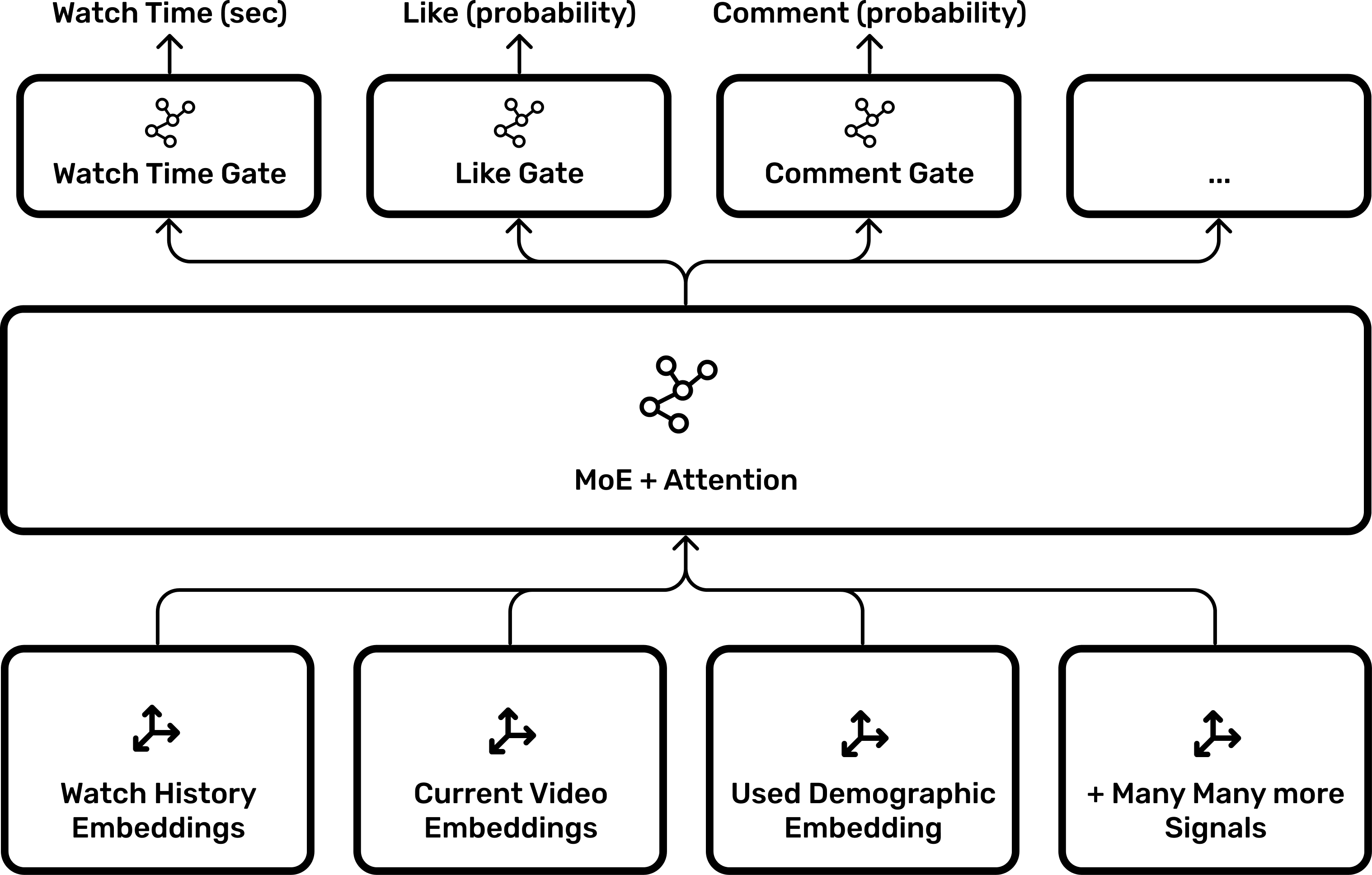
YouTube likely adopted the architecture described in their 2019 paper “Recommending What Video to Watch Next.”
Instead of a single dense neural network, the Ranking Model uses Mixture of Experts (MoE).

• The Experts: Sub-networks specialized in recognizing different patterns.

• The Gates: The model feeds into multiple “Gates,” each predicting a specific probability:

  • $$P(\text{Click}) P(\text{Watch Time}) P(\text{Like}) P(\text{Share}) P(\text{Dismiss})$$

Original article figure

The Weighted Score

The final score isn’t just watch time. It is a weighted sum of these gated outputs:

This brings us to the bleeding edge. Google is currently the only company with a natively multimodal LLM (Gemini) that accepts video input directly.

The Experiment

I conducted a latency test to validate if YouTube uses Gemini-style encoders:

1. Control: Upload a video file to Google Drive and ask Gemini to analyze it. Time: 6 minutes.

2. Test: Upload the same video to YouTube, then link it in Gemini. Time: <1 second.

The Implication

There is no physical way Gemini encodes 4K video in sub-second time. The only explanation is Caching.
The video tokens (embeddings) were likely generated by YouTube’s ingestion pipeline upon upload and stored. When Gemini requests the video, it retrieves the pre-computed embeddings.

This suggests that Gemini’s Video Encoder is now a component of the YouTube signal pipeline. The recommendation system doesn’t just know “tags” or “titles”—it fundamentally “sees” the video content.

Finally, we must account for active interference. YouTube acknowledges demoting “borderline content” (misinformation, flat earth, etc.).
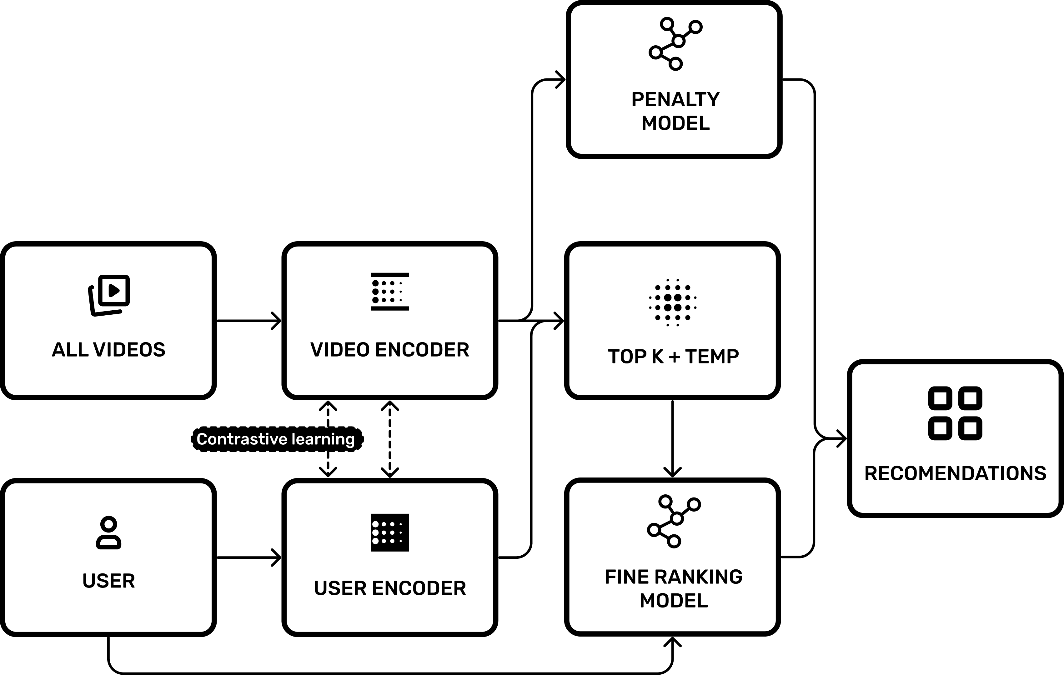
This is likely implemented as a Penalty Model: A separate classifier that scans the video embedding.

• If P(Misinfo)>Threshold, apply a negative weight to the final Ranking Score.

• This effectively creates a “soft ban” where the video exists but requires massive user signal to overcome the negative starting weight.

If the algorithm strictly adhered to the “Top-K Similarity” (finding the exact mathematical closest videos to the user), it would create a catastrophic user experience known as the Filter Bubble.

If you watch one tennis video, the model would calculate that the mathematically “closest” video is another tennis video. Eventually, your feed would become a loop of identical content. This maximizes short-term relevance but destroys long-term retention due to boredom.

The Solution: Stochastic Exploration

To solve this, YouTube likely borrows a concept from LLMs: Temperature.
Instead of deterministically picking the top 100 matches, the system likely introduces a “Fuzzy Edge” or randomness factor into the retrieval process.

• Exploitation: 90% of the recommendations are close matches (Tennis).

• Exploration: 10% are loose matches selected via a higher temperature setting (e.g., Pickleball, or Badminton).

This controlled randomness forces the user out of their local minima, allowing them to discover new interests and keeping the session dynamic.

Original article figure

The YouTube algorithm often feels like a mystery, but as we’ve seen, it is simply a reflection of the history of AI research. From the basic deep neural networks of 2016 to the multimodal power of Gemini today, the system has evolved from merely tracking clicks to fundamentally “seeing” and understanding the content of a video.

While we can’t know the exact code running on Google’s servers, the trail of research papers gives us a clear map of the territory. It is no longer a black box, but a complex, predictable machine built to solve a massive matching problem. As AI models continue to scale, we can expect this system to become even more precise, making the line between what we say we want and what the algorithm knows we will watch increasingly thin.

Watch the original YouTube demonstration ↗